Abstract Link to heading
I have been working on a project of creating my own Large Language Model, as I am huge fan of T5, or to be more concrete I recognize the added value of having an Encoder-Decoder architecture. The biggest challenge, at least in my opinion, in training an LLM is the sheer computational costs required to do so. I was originally planning to take the Encoder introduced by ColT5 but than I came across of M2 BERT and suddenly I went down the rabbit hole of Structured Matrices, Butterflies, Monarch and Hyeans.
Modern GPU Link to heading
Before we start, let’s take a look at an NVIDIA Tensor Core. It is a specialized compute core that allows for fused multiply-add operation. This means we can multiply two $4 \times 4$ and add to a third $4 \times 4$ matrix in a single operation. Now, why is this useful? it is just an 4 by 4 matrix, and I have huge matrices to multiply. Well, there is something called Block Matrix Multiplication.
Block Matrix Multiplication Link to heading
The idea is that we take a matrix and we chop it into smaller identically sized matrices. The actually computation works the same as the normal matrix multiplication, with the difference that we are now multiplying and adding together smaller matrices. (Multiplication and Addition)
Here is an example:
$$A = \begin{bmatrix} \begin{bmatrix} 1 & 2 \\ 3 & 4 \end{bmatrix} & \begin{bmatrix} 5 & 6 \\ 7 & 8 \end{bmatrix} \\ \begin{bmatrix} 9 & 10 \\ 11 & 12 \end{bmatrix} & \begin{bmatrix} 13 & 14 \\ 15 & 16 \end{bmatrix} \end{bmatrix}$$
$$B = \begin{bmatrix} \begin{bmatrix} 17 & 18 \\ 19 & 20 \end{bmatrix} & \begin{bmatrix} 21 & 22 \\ 23 & 24 \end{bmatrix} \\ \begin{bmatrix} 25 & 26 \\ 27 & 28 \end{bmatrix} & \begin{bmatrix} 29 & 30 \\ 31 & 32 \end{bmatrix} \end{bmatrix}$$
Three sulting matrix $C = AB$ is:
$$C_{11} = \begin{bmatrix} 1 & 2 \\ 3 & 4 \end{bmatrix} \begin{bmatrix} 17 & 18 \\ 19 & 20 \end{bmatrix} + \begin{bmatrix} 5 & 6 \\ 7 & 8 \end{bmatrix} \begin{bmatrix} 25 & 26 \\ 27 & 28 \end{bmatrix}$$
$$C_{12} = \begin{bmatrix} 1 & 2 \\ 3 & 4 \end{bmatrix} \begin{bmatrix} 21 & 22 \\ 23 & 24 \end{bmatrix} + \begin{bmatrix} 5 & 6 \\ 7 & 8 \end{bmatrix} \begin{bmatrix} 29 & 30 \\ 31 & 32 \end{bmatrix}$$
$$C_{21} = \begin{bmatrix} 9 & 10 \\ 11 & 12 \end{bmatrix} \begin{bmatrix} 17 & 18 \\ 19 & 20 \end{bmatrix} + \begin{bmatrix} 13 & 14 \\ 15 & 16 \end{bmatrix} \begin{bmatrix} 25 & 26 \\ 27 & 28 \end{bmatrix}$$
$$C_{22} = \begin{bmatrix} 9 & 10 \\ 11 & 12 \end{bmatrix} \begin{bmatrix} 21 & 22 \\ 23 & 24 \end{bmatrix} + \begin{bmatrix} 13 & 14 \\ 15 & 16 \end{bmatrix} \begin{bmatrix} 29 & 30 \\ 31 & 32 \end{bmatrix}$$
Resulting in: $$C = \begin{bmatrix}\begin{bmatrix} 322 & 338 \\ 580 & 608 \end{bmatrix} & \begin{bmatrix} 422 & 440 \\ 762 & 798 \end{bmatrix} \\ \begin{bmatrix} 994 & 1038 \\ 1290 & 1346 \end{bmatrix} & \begin{bmatrix} 1166 & 1218 \\ 1542 & 1606 \end{bmatrix} \end{bmatrix}$$
Because of block matrix multiplication (well there are more operations that work well with block matrices not just multiplication) we can take advantage of the NVIDIA Tensor Cores and speed up the computation.
Butterflies Link to heading
Before Butterflies we need to understand Structured Matrices and their significance. A structured matrix is a matrix that has a special structure that enables for faster, sub-quadratic $O(n^2)$ operations for dimension $n \times n$ in runtime and parameters.
Since this post is about Language Models, let’s make a brief pause and discuss Transformers. The core concept of transformers is the self-attention mechanism. Unfortunately, the self-attention mechanism is quadratic in the input sequence length, and replacing it with a more efficient version is an active area of research.
Butterfly Matrices Link to heading
Butterfly matrices are a super set of structured matrices, and we can view them as a product of block diagonal and permutation matrices.
Let $M \in B^{n}$ be a class of Butterfly Matrices, than we can express it recursively as:
$$ M = B_n \begin{pmatrix} M_1 & 0 \\ 0 & M2 \end{pmatrix} $$
- $B_n \in \mathcal{BF}^{(n,n)}$ is a Butterfly Factor
- $M_1, M_2 \in B^{(n/2)}$ are Butter Fly matrices but half of the size
Butterfly Factor Matrix Link to heading
A Butterfly Factor Matrix $\mathcal{BF}^{(n,k)}$ is a block diagonal matrix of size n and block size k, containing $\frac{n}{k}$ Butterfly factors $$ diag(B_1, B_2, \cdots, B_{\frac{n}{k}})$$
- $B_i \in \mathcal{BF}^{(k,k)}$
Butterfly Factor Link to heading
These are just block diagonal matrices, which means that we can partition the matrix into smaller matrices (blocks) with each block being an diagonal matrix.
$$ \mathcal{BF}^{(k,k)} = \begin{pmatrix} D_1 & D_2 \\ D_3 & D_4 \end{pmatrix} $$
- $D_i$ is a $\frac{k}{2}$ diagonal matrix
- $k$ is even
Benefits Link to heading
We already talked about block matrix multiplication, if we look once more at the recursive definition of Butterfly Matrices:
$$ M = B_n \begin{pmatrix} M_1 & 0 \\ 0 & M2 \end{pmatrix} $$
We see that we have an block diagonal matrix times a diagonal block matrix. Diagonal block matrices are great since there are a lot of zeroes, and we can ignore them. This promotes sparsity and computational efficiency at the same time.
Monarchs Link to heading
The main idea behind Monarch Matrices is to take two sparse matrices and multiply them together to approximate a dense matrix. And to make it as efficient as possible, we design the class of Monarch Matrices to be an product of two (Or more depending on the order) block diagonal matrices.
Order of p Monarch Matrix Link to heading
Let an $M^{N \times N}$ monarch matrix be defined as:
$$M = (\prod_{i=1}^p P_i B_i)P_0 $$
- $P_i$ is a bit-reversal permutation related to the base $\sqrt[p]{N}$
- $B_i$ is a block diagonal matrix with blocksize b
What does this tells us? If we take p block diagonal matrices and interleave them with a series of permutation matrices, we can approximate a dense matrix. Obviosly, choosing the right permutation matrices and block diagonal matrices is not trivial.
Order 2 Link to heading
Lets talk about a special case, where we have two block diagonal matrices:
$$M = PLPRP$$
- $L,R$ are block diagonal matrices
- it is common to set $L = R = (I_{\sqrt{N}} \otimes F_{\sqrt{N}})$
- $F_{\sqrt{N}}$ is an $\sqrt{N}$ Discrete Fourier Transform matrix
- $\otimes$ is the Kronecker product
- it is common to set $L = R = (I_{\sqrt{N}} \otimes F_{\sqrt{N}})$
- $P$ is a permutatin that maps $[x_1, \cdots, x_n]$ to $[x_1, x_{1+m}, \cdots, x_{1+(m-1)m}, x_2, x_{2+m}, \cdots, x_{2+(m-1)m}, \cdots, x_m, x_{2m}, \cdots, x_n]$
- this takes a vector of length n and reshapes it into an $b \times \frac{n}{b}$ matrix in row-major order, transposes it and flattens it in a vector
Connection to Butter Fly Matrices Link to heading
Why the hell did we need to talk about Butterfly Matrices? As it turn out, we can reexpress any Butterfly Matrix as a Monarch Matrix. Why is that? It turns out that we can express any diagonal block matrix as a block diagonal matrix using two permutation matrices from both sides. This property makes Monarch Matrices at least as expressive as Butterfly Matrices.
Monarch Mixer (M2) Bert Link to heading
That was maybe a bit of unnecessarily amount of theory, but now we can finally look into M2 Bert, which is an Attention and MLP free version of BERT.
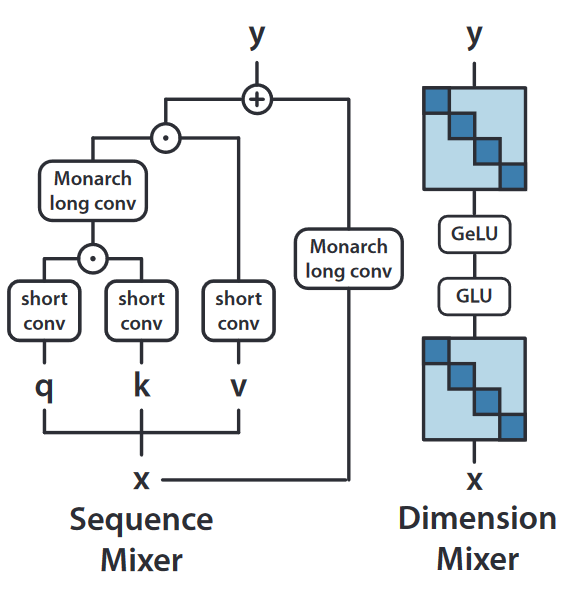
We have two parts:
- Sequence Mixer
- Dimension Mixer
Sequence Mixer Link to heading
Sequence Mixer performs short convolutions, this is just torch.nn.Conv1d, Monarch Long Convolutions.
Long Convolution and Hyenas Link to heading
First lets define convolution:
$$y_t = (h * u){t} \sum^{L-1}{n=0} h_{t-n} u_n$$
This is just a sum of element-wise multiplication of the filter $h$ and the input signal $u$. Unfortunately there is a catch. Generally the length of the filter is much shorter than the input signal. This implies that an explicitly defined convolution filter can only take into account the local context.
One way to overcome this is to use the implicit parametrization of convolution:
$$ h_t = \gamma_{\theta}(t) $$
In M2 Bert we are going to leverage this implicit parametrization and define the Hyena Filter as:
$$ h_t = Window(t) \cdot (FFN \circ PositionalEncoding)(t) $$
- $Window(t)$ is ExponentialModulation
class ExponentialModulation(OptimModule):
    def __init__(
        self,
        d_model,
        fast_decay_pct=0.3,
        slow_decay_pct=1.5,
        target=1e-2,

        modulation_lr=0.0,
        shift: float = 0.0,
        **kwargs,
    ):
        super().__init__()
        self.shift = shift

        max_decay = math.log(target) / fast_decay_pct
        min_decay = math.log(target) / slow_decay_pct
        deltas = torch.linspace(min_decay, max_decay, d_model)[None, None]
        self.register("deltas", deltas, lr=modulation_lr)

    def forward(self, t, x):
        decay = torch.exp(-t * self.deltas.abs())
        x = x * (decay + self.shift)

        return x
- $FFN$ is a Feed Forward Network and in our case we have and 2 layer MLP with Sinusoidal Activation Function
This is way to abstract, let’s look at an example:
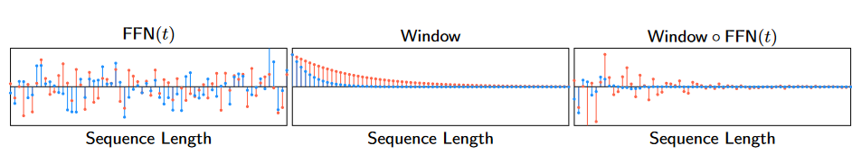
Having an long exponentially decaying part helps the model to select specific inputs at specific steps, combining it with high-frequency periodic activations (Sine) helps mitigating the low-frequency bias of neural networks. (Low frequency bias is a phenomenon where the model tends to learn smooth functions with small changes)
What is the deal with the Hyena anyway? Everything comes from the Hyena Hierarchy paper. In short, they take the ideas introduced at H3 and further generallize them, introducing the Hyena Operator.
Remarks Link to heading
What does this has to do with Monarch Matrices? Well, technically, we use Fast Fourier Transformation to perform the convolution, which gives us sub-quadratic time complexity, for more information check out MonarchMixerSequenceMixing
Dimension Mixer Link to heading
In the Dimension Mixer, we take the output from the Sequence Mixer and we mix the information across the model dimension. This is done by multiplication with a Block Diagonal Linear neural network layer. The weights of this layer are just a Block Diagonal Matrix. Here is a simplified Python implementation of the Block Diagonal Linear Layer:
import torch
import numpy as np
from torch import nn

class BlockDiagonalLinear(nn.Module):
  def __init__(self, blocks=4, hidden_size, intermediate_size):
    self.blocks = blocks
    self.hidden_size = hidden_size
    self.intermediate_size = intermediate_size

    in_size = hidden_size // blocks
    intermediate = intermediate_size // blocks

    self.wweight = nn.Parameter(torch.zeros(blocks, in_size, intermediate))
    self.reset_parameters() # To Kaiming weights

  def forward(self, x):
    batch_shape, n = x.shape[:-1], x.shape[-1]
    batch_dim = np.prod(batch_shape)
    nblocks, q, p = self.weight.shape
    assert nblocks * p == n
    x_reshaped = x.reshape(batch_dim, nblocks, p).transpose(0, 1)
    out = torch.empty(batch_dim, nblocks, q, device=x.device, dtype=x.dtype).transpose(0, 1)
    out = torch.bmm(x_reshaped, self.weight.transpose(-1, -2), out=out).transpose(0, 1)
    return out.reshape(*batch_shape, nblocks * q)
The pseudo code for the Dimension Mixer forward pass is:
y = BlockDiagonalLinear(blocks=4, hidden_size=768, intermediate_size=3072)(x)
y = nn.GELU(approximate='none')(y)
# y = nn.Dropout(p=0.1)(y) # In general we use dropout only during training
y = BlockDiagonalLinear(blocks=4, hidden_size=3072, intermediate_size=768)(y)
y = nn.LayerNorm()(y)
return y
Finishing it up Link to heading
Since we have defined the Sequence and Dimension Mixer, we can now define the M2 Bert Layer:
class M2BertLayer(nn.Module):
  def __init__(self, hidden_size=768, intermediate_size=3072):
    self.sequence_mixer = MonarchMixerSequenceMixer(hidden_size=hidden_size)
    self.dimension_mixer = DimensionMixer(hidden_size=hidden_size, intermediate_size=intermediate_size)

  def forward(self, x):
    x = self.sequence_mixer(x)
    x = self.dimension_mixer(x)
    return x
And to get a BERT model we just stack a couple of M2 Bert Layers, and that is it.
Performance Link to heading
The biggest benefit of M2 Bert is that it achieves 9x the throughput for a sequence length of 4096, and it achieves an 27% parameter reduction while maintaining the same accuracy. This allows us to train significantly larger models with the same resources.
Conclusion Link to heading
In the past, I read a lot of research about how to speed up or increase the context size of the Encoder part of T5. M2 BERT is a fresh take on to do this, and I cannot wait to see how it will work out in practice. In the meantime I reignited my interest in State Space Models and discovered Hydra which is a Bidirectional extension of Mamba. There is this new trend of combining Attention and State Space Models, an example of which is Samba. In my personal opinion the combination of Hydra and M2 Bert could lead to an exremely powerful and efficient model.