Abstract Link to heading
In the last two years there has been a surge of Large Language Models. This is understandable, since LLMs are amazing at generating text, and a lot of things can be viewed as text. However, generation is not always all we need - sometimes we want to have semantically rich representations. In general, LLMs are not the best tool to get semantically rich representations, and even today models like BERT are used to achieve state of the art text embeddings. A natural question is to ask why BERT is so much better at embeddings than LLMs? Here are the two main reasons:
- Causal vs bidirectional attention, in causal attention the contextual representation of a token is determined by the current token and all (or a window with sliding window attention) previous tokens. With bidirectional attention, we also allow influence from future tokens. This makes intuitive sense - if we want to see importance, or meaning of a word in a sequence, it makes sense to take into account words that come before and after.
- Next token prediction vs Masked Token Prediction, decoder models are trained to predict the next token given the previous. This is obviously very efficient if we want to generate semantically valid text. Encoder models are trained on Masked Token prediction, which means we replace a random sample (usually 15%) of tokens with a special [MASK] token. Its goal is to recover the masked token, and it is done by leveraging information from the neighborhood of the masked token.
It is not hard to see that causal models are meant to be good at predicting future tokens, while encoder models are designed to capture information about their surroundings. A natural question to ask is: “If Bidirectional models are so good why do we not stick to them, and train them to get better embedding models?”. Again there are a couple of reasons:
- Sample efficiency of LLMs, let’s start here with an example sentence: “I think this article is really cool.”. It does not matter if this is true or not, we can show how a causal LLM is trained: $$ p(., “I”) $$ $$ p(.| “think”, “I”)$$ $$ p(.| “this”, “think”, “I”)$$ $$ p(.| “article”, “this”, “think”, “I”)$$ $$ p(.| “is”, “article”, “this” ,“think”, “I”)$$ $$ p(.| “really” ,“is”, “article”, “this” ,“think”, “I”)$$
We can see that a single sentence produces multiple training examples, here $p(.|)$ says we want to observe the next word. (Sure LLMs operate on tokens not words but the intuition still applies).
For Masked Token Prediction the examples would be:
$$ p([MASK]| “I”, “think”, “this”, [MASK], “is”, “really”, “cool”) $$ $$ p([MASK]| “I”, “think”, “this”, “article”, “is”, “really”, [MASK]) $$
Here we want to predict [MASK], given the surrounding, and usually we use a sentence only a couple of times. Technically we could reuse the sentence as many times as we want, but it is usually not done.
- LLMs are more useful, here we may argue a bit, but maybe not. ChatGPT, Claude, or other Generative models, have made an impact on knowledge workers, and have potential to transform many aspects of work. On the other hand embedding models are useful but they are constrained to certain subjects like similarity detection, information retrieval and classification, all useful but the overall impact is somewhat less profound.
Let’s recap the text above: LLMs are more efficient to train and are more flexible ultimately yielding them more useful, but for some special cases we need an encoder model to get rich representations. A natural question is: “Can we train an LLM and somehow make it so that it can produce rich semantic representations?”. The answer is of course we can, and we will cover the current state of the art how to do it:
- LLM2Vec: Large Language Models are Secretly Powerful Text Encoders
- NV-Embed
- Large Language Models Are Overparameterized Text Encoders, this is a bit different than the papers above and it focuses on reducing the runtime costs of newly created models.
Remark Link to heading
There is also a family of Encoder-Decoder models like T5. These models are excellent at providing rich embeddings and they are great at generating text. So are they perfect? Yes they are, but (of course there is a but) they are way less efficient if you use them as a conversational agent. In a decoder only language model, you can cache the previous token representation, since they do not change if we keep adding tokens to the end. With encoder-decoder models, we need to always reevaluate the entire input before we pass to the decoder, even if we only add a single token at the end. Ok so this is not 100% true, we could append the extra tokens just to the decoder, but that will limit the expressivity of the model.
Sequence Embeddings Link to heading
Before we look into the main research papers, we have to clarify what a sequence embedding is. It is a function that takes an arbitrary long input and transforms it into a fixed length output.
$$ f: X \in R^{l \times d} \rightarrow Y \in R^d $$
- $l$ is the length of the original sequence
- $d$ is the dimension of this sequence
In human language, we take an arbitrary long text and we transform it to a fixed sized vector. A common way to get a sequence embedding is just to average individual entries out, however with tokens this is not very fortunate, since different tokens can contribute more to an overall representation. A better way is to take a weighted average, where we use a learnable weight function.
LLM2Vec Link to heading
LLM2Vec is an unsupervised approach that can transform any decoder-only LLMs into a strong text encoder. This is done without any expensive synthetic data in a parameter efficient way, and it works in 3 steps.
Steps Link to heading

- Enable bidirectional attention
- Masked next token prediction
- Unsupervised [[Contrastive Training|Contrastive Learning]]
Enable Bidirectional Attention Link to heading
At the beginning of this article we established why causal attention mask is not the best option if we need a rich embedding. Because of this, the first step in LLM2Vec is to replace the attention mask with a bidirectional (all ones) mask. If we use FlashAttention the following will make the trick:
flash_attn_func(q, k, v, causal=False, window_size=(-1, -1)):
Later in the benchmarks, we are going to see that changing from causal to bidirectional attention won’t really help; actually it will worsen the model’s performance. The reason is that the model does not really know what to do with future information.
Masked Next Token Prediction (MNTP) Link to heading
As mentioned above, we need to teach the model to leverage information from future tokens. To do that we train it on Masked Next Token Prediction objective. MNTP is similar to Masked Language Modeling, with one key distinction: to predict the masked token at position $i$, we take the representation at the previous token $i-1$ and not the masked position itself.
Unsupervised Contrastive Learning Link to heading
In the previous step we healed the model - it is no longer confused about what these new tokens are about, and we have a good word level model. But since LLMs were not trained to capture the semantics of a whole sentence, we fill this gap by applying Contrastive learning. The key idea behind contrastive learning is that we want to pull the semantic representations of similar samples/sentences closer together while pushing dissimilar ones farther apart. Here we follow the recipe introduced by SimCE, and we need positive and negative samples. Positive samples are generated from the sentence itself by applying a random dropout mask with dropout probability 0.3 and we generate exactly two samples. Dropout probability 0.3 is rather high; usually researchers leverage 0.1 when training bidirectional models with contrastive objective. Negative samples are simply other examples in a given mini-batch.
Training Link to heading
We have our 3 steps, from this Masked Next Token Prediction and Unsupervised Contrastive learning introduce objectives that require training. As a dataset, English Wikipedia is chosen, mainly because the underlying model should be already trained on it. For both objectives we leverage LoRA, which we merge back into the model. As for compute, it requires a single 80GB A100 GPU for around 5 hours, which makes LLM2Vec compelling for individuals and academic institutions.
Results Link to heading
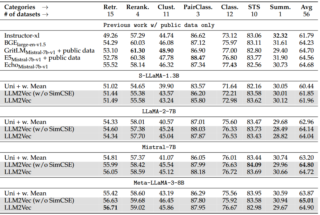
The researchers applied LLM2Vec to Mistral-7B, S-LLama-1.3B and Llama-2-7B and here are the results:
Word Level Link to heading

We have two baselines, the first is deBERTa-v3-large (dashed lines, and it is a 418M parameter model, however 131M are the initial embeddings) and the embedding produced by a plain causal model (full line).
In general, swapping causal attention for bidirectional hurts the performance, but not in case of Mistral. Here it is theorized that it may have been trained in some of its pretraining phases with bidirectional attention.
If we include MNTP we observe increased performance since the model was taught to leverage the bidirectional information. Contrastive learning actually hurts the performance a bit; this makes sense since its contribution is to get a better sentence model and it is not needed for a word model.
Sentence Level Link to heading
Here the baseline is a BERT model that was trained in the SimCSE paper and we also explore various pooling methods over individual token representations.

The results follow similar trend as in Word Level tasks: bidirectional attention without finetuning hurts the performance, but not for Mistral. The best results are achieved by applying all 3 steps with weighted mean pooling.
Further Finetuning for MTEB Link to heading
To further evaluate the performance the authors use the MTEB: Massive Text Embedding Benchmark here is the Leaderboard from Hugging Face where you can check the latest and greatest.

NV-Embed Link to heading
If you checked the leaderboard (well, it depends when you are reading this post), you noticed that NV-embed was in first place. Because of this, we cannot really ignore it. NV-Embed shares a lot of similar design decisions with LLM2Vec - both swap causal for bidirectional attention, both finetune the resulting model. However, NV-Embed only does Contrastive learning. The biggest difference is how they pool individual token representations into a single embedding - NV-Embed introduced a novel technique called Latent Attention.
Latent Attention Link to heading

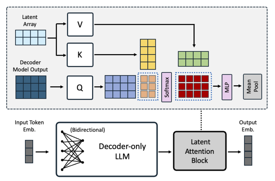
Latent Attention is just cross attention defined as:
$$O \in R^{l \times d} = \text{softmax}(QK^T)V$$
- $Q \in R^{l \times d}$ is the output from the last attention layer with $l$ the sequence length and $d$ the hidden dimension.
- $K = V \in R^{r \times d}$ are trainable parameters “dictionary”, which is used to obtain better representations, $r$ is the number of latents in the dictionary.
Once we have our output $O$ we transform it with two linear layers each with GeLU activation, followed by mean pooling to get the final embedding.
Intuition Link to heading
Let’s put this into more human-like words: our latent K,V vectors are learned during training, and they are independent of the input during inference (this makes dictionary actually a great name). Since Q comes from the actual input sequence, we can view the whole latent attention as an average over the latent dictionary weighted by the input sentence. The two MLPs perform channel mixing (mixing along the latent dimensionality of individual entries in the output sequence). At the end, we can just do mean pooling since we already have a weighted mixture of individual tokens from the attention operation.
Training Link to heading
We need to perform training since the model does not know what to do with the extra token information that it gets from the bidirectional attention, and we need to learn the latent dictionaries for the latent attention. The training is done in 2 stages:
Contrastive Training Again we follow the SimCE recipe but with the following modifications: we do not generate extra positive samples with dropout, there is just one. As for negatives, we have in-batch negatives and hard negatives. Hard negatives are negative samples chosen for a given sample.
Contrastive Instruction Tuning
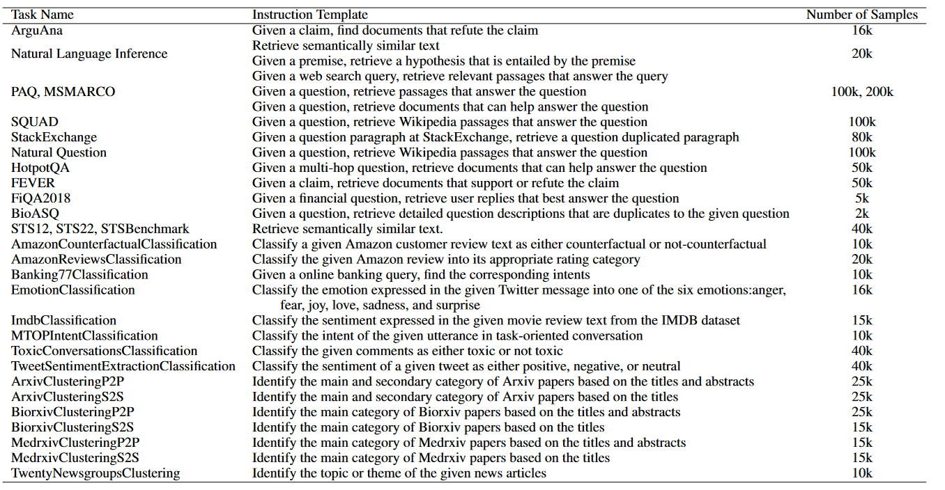
The instruction following capacity of LLMs makes them extra compelling. By introducing prompts to embedding models, we can steer the embedding more towards our needs. Since we want to use embedding not just for retrieval but also classification, clustering and other non-retrieval tasks, we include extra training data for this purpose.
Here is the complete list of possible prompts:

During instruction tuning we also do not use in-batch negatives, mainly because a single batch may contain actual samples from the same class and it will mislead the model.
Experiments Link to heading
The authors build their model on top of Mistral 7B, where the latent attention has 512 latents, and the resulting sequence embedding is 4096 long. As with LLM2Vec, the training was done using LoRA, for NV-Embed with rank 16, alpha 32 and Dropout 0.1.
MTEB results Link to heading
And here are the official results for MTEB. Results are taken directly from the paper. Currently, there is a v2 model on top of the charts, which leverages NV-Retriever to mine the hard negatives.

Large Language Models are Overparameterized Text Encoders Link to heading
Maybe you already noticed, if we derive an encoder model from an LLM, they tend to have a lot of parameters especially if we compare them to existing state of the art - they are even 20x larger. Their size makes them significantly slower and more expensive to run. A common approach to reduce model size is to start dropping layers.
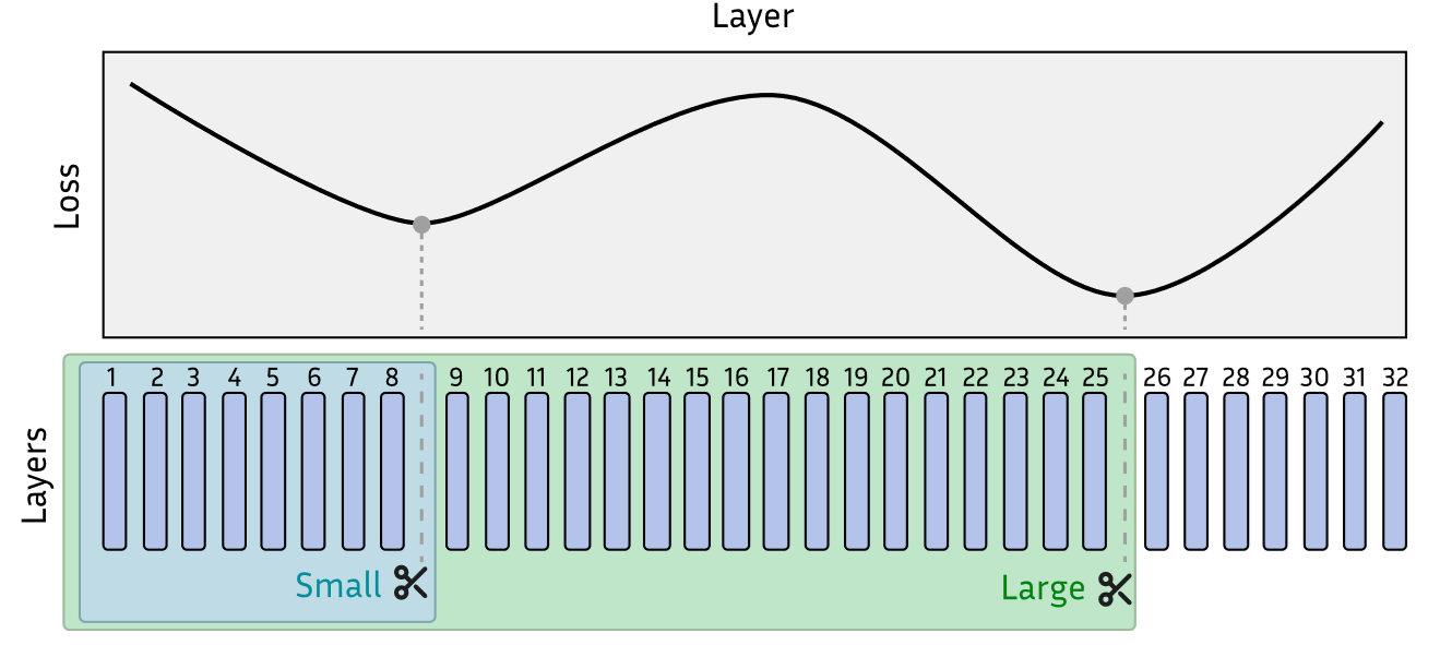
However not all layers are equal, it is theorized that the lower layers in Large Language Models are responsible for extracting the necessary information from the underlying input and the higher levels are responsible for generating meaningful text, that is predicting the next token. Since we are more interested in having efficient embeddings, we can prune the top layers, but how much is too much?

The picture above has two local minima, and we can use that to create two models: one that is large but retains most of the LLM’s performance and one that has a larger performance drop but is small and cheap to run.
$L^3$ Prune Link to heading
$L^3$ prune is a method that automatically determines the optimal cutoff point. For more information, here is the forked source code

We can clearly see that we can chop off the upper 10-20% of layers and see virtually no performance drop. We can push it further and remove around 70-80% of the top layers and see some minor drop while still maintaining excellent performance.
Final Thoughts Link to heading
Since my main interests lie more in understanding tasks than in generation problems, this research was very needed. For a very long time, I thought that I would need to pretrain my own embedding model; however, as we all know, that is expensive and generally discouraged. Right now, I see that I can create a powerful embedding model, in my example from Qwen-2.5 Coder. What would be extremely nice to see is if I could take the ideas from NV-Embed (mainly because it is the latest research already leveraging ideas from LLM2Vec, however I still see the need to have a word-level pretraining step) and fuse it with Matryoshka Representation Learning to get a leaner final representation.