Abstract Link to heading
In the last RL-Bite I wrote about Bellman’s Equations and the Value Function and now we will figure out how we actually apply these equations to compute the Value Function!
Known World Model Link to heading
Let’s start with the simple case, and make an assumption that the underlying World Model of the Markov Decision Process is known, and we have finite discrete states. If we include that the Discount Factor $\gamma < 1$, we can find the Optimal Value function exactly using:
- Dynamic Programming
- Linear Programming
However, the computational complexity in both cases is polynomial in the size of possible states and actions and we may struggle because of the Curse of Dimensionality if this space is too large. In these cases we need to use approximate variants: Approximate Dynamic Programming or Approximate Linear Programming.
Value Iteration Link to heading
At the core, Value Iteration leverages Dynamic Programming, the update equation is:
$$ V_{k+1}(s) = \max_a [ R(s, a) + \gamma \sum_{s^{\prime}} p(s^{\prime}|s, a) V_k(s^{\prime}) ]$$
Where we apply Bellman’s Backup, with $V_k$ the current estimate of the Value function.
The benefit of this approach is that it contracts, which means that with each iteration the error decreases:
$$ \max_s |V_{k+1}(s) - V_{\star}(s)| \leq \gamma \max_s |V_k(s) - V_{\star}(s)|$$
In practice we stop if we get close enough to the Optimal Value Function, and again we reach for the Bellman’s Equations to extract the Optimal Policy.
Real-time dynamic programming (RTDP) Link to heading
Real-time Dynamic Programming is a modification of Value Iteration, where we consider only a subset of states we are interested in:
$$ V_{k+1}(s) = \max_a E_{p_s(s^{\prime}|s,a)}[ R(s, a) + \gamma V_k(s^{\prime}) ]$$
- here we have $p_s(s^{\prime}|s,a)$ this is just the transition matrix of the MDP
- $R(s,a) = -1$ for the states we are not interested in
Policy Iteration Link to heading
Again a Dynamic Programming approach to compute the optimal policy $\pi_{\star}$ by searching the space of deterministic policy where we repeat two steps until we converge. These steps are:
- Policy Evaluation The idea is to compute the value function for the current policy $\pi$ as $v(s) = V_{\pi}(s)$, here $v$ is a vector indexed by state, $r(s) = \sum_{a} \pi(a|s)R(s,a)$ is the reward vector and $T(s^{\prime}|s) = \sum_{a}\pi(a|s)p(s^{\prime}|s,a)$ is the state transition matrix. With this we express the Bellman’s Optimality Equations in matrix form:
$$ v = r + \gamma Tv $$
This is a system of equations with $|S|$ unknowns and we can solve it by using matrix inversion:
$$v = (I - \gamma T)^{-1} r$$
Alternatively we can use Value Iteration $v_{t+1} = r + \gamma T v_{t}$ until it converges
- Policy Improvement
In this step we have a policy $\pi$ with a value function $V_{\pi}$, this can be used to derive a better policy $\pi^{\prime}$ as follows:
$$ \pi^{\prime}(s) = \arg \max_{a}{ R(s,a) + \gamma E[V_{\pi}(s^{\prime})] }$$
Given the Policy Improvement Theorem we are guaranteed that $V_{\pi^{\prime}} \ge V_{\pi}$
Summary Link to heading
The process can be summarized as: $$ \pi_0 \xrightarrow{E} V_{\pi_0} \xrightarrow{I} \pi_1 \xrightarrow{E} V_{\pi_1} \dots \xrightarrow{I} \pi_* \xrightarrow{E} V_*$$
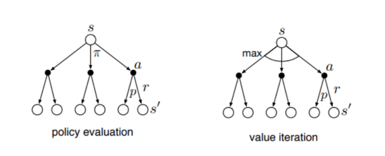
Comparison of VI and Policy Iteration Link to heading
Policy Iteration and Value Iteration are extremely similar, the difference is that in Policy Evaluation we average over all actions according to the policy, while in VI we take the maximum over all actions, the following 2mage gives a nice summary:
Unknown World Model Link to heading
Until now the Agent had access to the underlying world model, here we can agree, that this is not realistic and we will focus on the case where the Agent only observes samples produced by the environment.
$$(s’ , r) \sim p(s’,r|s,a) $$
Luckily for us this is enough to learn an Optimal Value Function.
Monte Carlo Estimate Link to heading
This can be also known as policy rollout, and the idea is that we take actions according to the policy (until we reach an absorbing state, alternatively the discount factor forces the rewards to zero), until we reach an end, and average out the discounted rewards. We use this average to update the estimated value function:
$$V(s_t) \leftarrow V(s_t) + \eta [G_t - V(s_t)]$$
High Variance Link to heading
As with other Monte Carlo methods they tend to have High Variance. Why is this the case? First each time we unroll a trajectory we work with a stochastic state transition function, and we need to sum up a lot of random rewards. This process is then repeated multiple times and we take an average at the end. Summing and averaging a lot of random variables is noisy!
Temporal Difference (TD) Learning Link to heading
This is an alternative to Monte Carlo Estimate, that promises to be more efficient. The idea is that we incrementally reduce the Bellman’s Error each time by making a single state transition: $(s_t, a_t, r_t, s_{t+1})$ with $a_t \sim \pi_{s_t}$. This can be used to estimate $V(s_t)$ as:
$$ V(s_t) \leftarrow V(s_t) + \eta [r_t + \gamma V(s_{t+1}) - V(s_t)]$$
- $q_t = r_t + \gamma V(s_{t+1}) \approx G_{t:t+1}$ - this is the one step Reward To Go
- $\delta_t = r_t + \gamma V(s_{t+1}) - V(s_t) = q_t - V(s_t)$ this is the TD Error
Parametric Form Link to heading
We can reexpress the equation above as:
$$ w \leftarrow w + \eta [r_t + \gamma V_w(s_{t+1}) - V_w(s_t)] \nabla_w V_w(s_t)$$
From this it should be obvious that it is a special case of Monte Carlo Estimate, where we do just one step. And it looks like Gradient Descent but it is not, it is bootstrap.
Convergence Link to heading
There is some good news: for the tabular case this is guaranteed to converge to the correct value function. The bad news is that if we use non-linear function approximators it may diverge.
Connection to Bellman’s Backup Link to heading
TD learning is a technique that uses sampled transitions to approximate the Bellman’s Backup. Giving us an approximate way to achieve the optimal Value Function.
Combination of MC and TD Link to heading
It is evident that MC and TD are very similar, where TD is essentially MC but with only one step look ahead and we can combine these approaches, by approximating the n-step return as:
$$G_{t:t+n} = r_t + \gamma r_{t+1} + \dots + \gamma^{n-1} r_{t+n-1} + \gamma^n V(s_{t+n}) $$
The update rule for TD becomes:
$$ w \leftarrow w + \eta [G_{t:t+n} - V_w(s_t)] \nabla_w V_w(s_t)$$
TD($\lambda$) Link to heading
This is a special case for MC + TD, where we do not specify how far we want to do a lookup but we take a weighted average of all possible values, this average is geometric, so we can sum even infinite long lookaheads:
$$G_t^\lambda = (1 - \lambda) \sum_{n=1}^\infty \lambda^{n-1} G_{t:t+n}$$
- $\lambda \in [0,1]$
- if we set it to $0$ we get plain TD learning
- if we set it to $1$ we get regular MC Estimation