Abstract Link to heading
Let’s talk a bit about Model-Based Reinforcement Learning. The idea is that our RL Agent not just learns a policy to follow or/and a value function (Q function) but also tries to model the environment it is in. This is done by learning the transition dynamics $p(s’|s,a)$ (also known as World Model) and a Reward function $\hat{R}(s,a)$. Once we have our world model, we can use it to simulate data and learn the model’s policy on the simulations. So here you may ask why the hell this is useful? First, Sample Efficiency! We are able to generate extra data to use during the training. Second, in some cases it is super expensive to explore the environment directly (imagine building a robot performing surgery! right). In practice, how we train these models is way more interleaved; we do a bit of model learning, then policy improvement, then back to model learning and so forth. Why so? Again, this goes back to the Deadly Triad, where we use the model itself to improve itself, where we end up in this self-reinforcing feedback loop making everything just worse.
Decision-time planning Link to heading
Before going into Monte Carlo Tree Search, let’s generalize it a bit. So what is decision-time planning? Well, before an agent makes a step, it does a bit of planning ahead. This is done by taking a known (or learned ahead) world model and exploring actions it can take, leading to new states, with further potential actions to take. Since this is a problem where the complexity is exponential, we usually bound the maximum exploration depth (usually denoted $d$), and the approach described is also known as receding horizon control. Once we’ve expanded the full tree, at every leaf we then compute the reward-to-go (this is the total reward that we would get if we start at the starting node $s_t$ and we walk all the way down to a leaf), and we choose the trajectory which yields the highest total reward (so this approach is also known as forward search
Optimizations Link to heading
Exponential is bad, so let’s look into how to make it more efficient:
- Branch And Bound, this is a heuristic where we eliminate walking down unfavorable paths. It requires a lower-bound on V and upper-bound on Q. In each state we visit, we order the actions we can take based on their upper-bound; if we find actions that are less than the current best lower bound, we prune it from the tree and we continue this until we hit a leaf node, where we return the lower bound
- Sparse Sampling, to reduce the states we need to explore, at each state we sample a set of actions we can take. Yes, we may miss the optimal path.
- Monte Carlo Tree Search
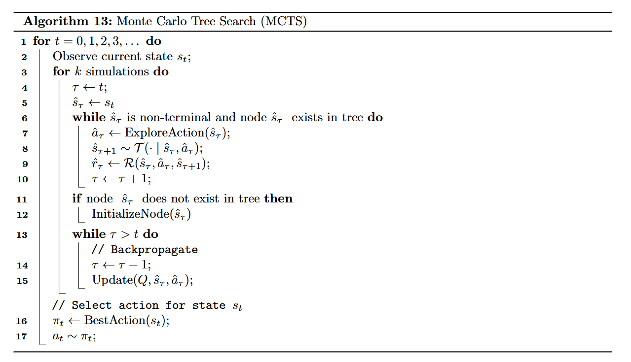
Monte Carlo Tree Search Link to heading
As before, we start at a root node $s_t$ and we perform $m$ Monte Carlo Rollouts to estimate $Q(s_t, a)$ and return the best action: $a = \arg \max_a Q(s_t,a)$ or distribution of actions (softmax). During the rollout we track how many times we have tried each action $a$ in each state $s$ using a counter $N(s,a)$
The rollout has the following steps:
- If we have not visited $s$ we initialize $N(s,a)=0$ and $Q(s,a)=0$ and we return the estimated value function ($U(s)$)
- If we have visited, we pick the next action to explore from state $s$; here we need to pick every action at least once
- Once we’ve taken each action $a$ exactly once, we then use an Upper Confidence Bound (UCB) to select subsequent actions:
$$ a = \arg \max_{a} Q(s, a) + c \sqrt{\frac{\log N(s)}{N(s, a)}}$$
- $N(s) = \sum_a N(s,a)$
- and we then sample the next state $s’ \sim p(s’|s,a)$
- Update the Q function using Temporal Difference (Bellman’s Update) $$ Q(s, a) \leftarrow Q(s, a) + \frac{1}{N(s, a)}(u - Q(s, a))$$
- We increment $N(s,a)$
Application Link to heading
The algorithm is not too complex, let’s look at a simplified overview of where it was applied and how:
AlphaGo and Extensions Link to heading
AlphaGo is just the application of MCTS to a two-player, zero-sum symmetric game
$$ p^{\pi}(s’|s, a^{i}) = \sum_{a^{j}} \pi(a^{j}|\psi(s)) p(s’|s, a^{i}, a^{j})$$
- $i$ is the main player and $j$ is the opponent
AlphaZeroGo, AlphaZero Link to heading
We introduce a Neural Network in MCTS to compute $(v^s, \pi^s) = f(s;\theta)$
- $v^s$ is the expected outcome of the game from state $s$ (+1, -1, 0) (win, loss, draw)
- $\pi_s$ is the policy that gives a distribution over actions for state $s$, and is used internally by MCTS to give additional exploration bonus to the most likely actions
The overall loss: $$ L(\theta) = E_{(s, \pi_{s}^{MCTS}, V^{MCTS}(s)) \sim D} [ (V^{MCTS}(s) - V_{\theta}(s))^{2} - \sum_{a} \pi_{s}^{MCTS}(a) \log \pi_{\theta}(a|s) ]$$
- $ D = { (s, \pi_{s}^{MCTS}, V^{MCTS}(s)) }$ is the dataset collected from a MCTS rollout started at state s
- $\pi_{s}^{MCTS}(a) = [ N(s, a) / (\sum_{b} N(s, b)) ]^{1/\tau}$ this is a distribution over actions at the root node s with $\tau$ is the temperature
- $V_{s_{t}}^{MCTS} = \sum_{i=0}^{n-1} \gamma^{i} r_{t+i} + \gamma^{k} v_{t+i}$ this is the n-step reward-to-go starting at $s_t$
MuZero and Extension Link to heading
AlphaGo assumes that the world model is known, whereas in MuZero we learn it. The model is learned by training a latent representation (embedding function) of the observation $z_t = e_{\phi}(o_t)$, and learning the corresponding latent dynamics model: $$ (z_t, r_t) = M_{w}(z_t,a_t) $$
The goal of the World Model is to predict the immediate reward and future reward of MCTS to compute the optimal policy
The total loss is: $$L(\theta, w, \phi) = E_{(o, a_{t}, r, o’, \pi_{z}^{MCTS}, V_{z}^{MCTS}) \sim D} { (V^{MCTS}(z) - V_{\theta}(e_{\phi}(o)))^{2} - \sum_{a} \pi_{z}^{MCTS}(a) \log \pi_{\theta}(a|e_{\phi}(o)) + (r - M_{w}^{r}(e_{\phi}(o), a_{t}))^{2} }$$
It has some extra terms to measure how well it predicts the observed rewards, and we optimize it with respect to:
- policy/value parameters $\theta$
- model parameters $w$
- embedding parameters $\phi$
Extensions Link to heading
Some notable extensions are:
- Stochastic MuZero, for stochastic environments
- Sampled MuZero, for large action spaces