Source

• Paper link: https://openreview.net/pdf?id=R8SolCx62K
• Source Code: https://github.com/hedongxiao-tju/SGRL

Abstract

Contrastive Learning (CL) is one of my favorite techniques, it is a self-supervised approach for learning latent representations with a special property: Similar elements have representations that are closer together and elements that are different are farther from each other. The paper: Exploitation of a Latent Mechanism in Graph Contrastive Learning Representation Scattering takes a very novel approach to CL and it gives a nice theoretical foundation of CL and Graph!

Representation Scattering

First what is Representation Scattering? The idea is that we learn a representation subspace, where individual entries are uniformly distributed in this subspace. Why is this useful? Without trying to cover the whole subspace, we may end up with hot-spots, where many entries live in, and waste uninhabited areas. This is suboptimal since we tend to use this subspace to compare entries and since we fail to cover the space evenly the whole distance will be extremely biased.

Graphs

Let’s elaborate on two constraints that are especially useful for Graphs in terms of Scattering:

1. Uniformity, this is just the thing from above, we try to cover the representation space uniformly.
2. Center away, so graphs are made of nodes and edges, the idea of center away, that the individual nodes of a given graph, should be centered around a Center Node (later we look into how to compute this) and nodes that are connected should be closer to each other than those that are not.

Graphs and other CL Approaches

Current research, in terms of CL and Graphs is more-or-less about 3 ideas:

1. DGI like methods
2. InfoNCE like methods
3. BGRL like methods

All of these approaches connect to Graph Representation Scattering, at least to some degree.

DGI

In DGI we need negative samples (this is a common theme in CL) they are constructed by corrupting (random node permutations) the original Graph. The positive samples are local patches (subgraphs) of the original graph. Because of this we have two distributions: original and noise. Where we maximize the Jensen Shannon Divergence (JSD) between the original distribution and the corrupted distribution. (JSD is just an alternation of KL divergence which is smooth and symmetric)

The connection to Representation Scattering is that: DGI tries to distinguish between the local semantics of nodes within the original graph and its mean, which correlates with representation scattering.

InfoNCE

In InfoNCE like approaches we choose an anchor point (this is a node in the Graph we want to learn representations for). We draw positive samples by using Graph augmentation methods (we do slight changes to the graph), and negative samples are in-batch negatives (or hard-negatives). The model is then trained by Contrastive Loss where we measure the cosine distance between the positive samples and anchor point, where we want this distance to be small and the same with negative samples but we want to maximize the distance.

The connection to Representation Scattering is more obvious, we have a center and we want nodes to be close to this center and the negative samples should force the individual representations to cover the whole subspace. Actually InfoNCE loss serves as an upper bound for representation scattering loss, however it is not perfect since the need of negative samples may introduce bias (false negatives) resulting in collapse of the representations subspace (super fancy words, in human language we end up with hot-spots).

BGRL

BGRL is inspired by the BYOL (Bootstrap Your Own Latent) method from computer vision. It avoids using explicit negative samples. Instead, it trains two neural networks – an online network and a target network – and the online network tries to predict the target network’s representation of a different augmented view of the same input. Where the target network provides “better” representations, which the online network learns to predict.

The connection to Representation Scattering is the use of Batch Normalization (BN) in BGRL methods (it is also shown that leaving out BN drastically reduces the accuracy). A reminder in BN we technically Normalize the data, but instead of having zero mean and unit variance we learn a parameter for the mean and variance, from this it is obvious that BN is a Center Away like constraint, however it is not perfect since it is indirect without explicit guidance, resulting in nonuniform coverage of the hyperspace.

Representation Scattering Mechanism (RSM)

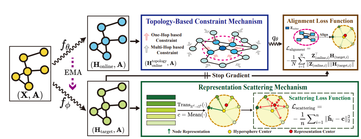
Let’s talk about how do we actually achieve Representation Scattering in a Graph:

Methodology

We have two core components:

1. Representation Scattering Mechanism (RSM)
2. Topology Based Constraint Mechanism (TCM)

Where SRM ($f_{\varphi }\to H_{target}$) and TCM $(f_{\theta }\to H_{online})$ are represented as two distinct encoders each with different parameters, each producing their own embedding, each serving a different role.

RSM

The first encoder: $f_{\varphi }\to H_{target}$ produces the first embedding. By taking the mean of $H_{target}$ we produce the Scattering Center (c) for all the nodes in the Graph that the nodes belong to. Parameters $\varphi$ are carefully updated in a way that we want to push away the individual node representations from the center:

$\widetilde{h_i}=Tran{s}_{R^d\to S^k}(h_i)=\frac{h_i}{Max(||h_i|{|}_2,ϵ)},S^k=\{\widetilde{h_i}:||\widetilde{h_i}|{|}_2=1\}$

• individual node representations $h_i$ are projected from the original space $R^d$ to a subspace $S^k$
• $ϵ$ is a small value so we do not divide by zero
• $||\widetilde{h_i}|{|}_2=({\sum }_{j=1}^k{\widetilde{h_{ij}}}^2{)}^{\frac{1}{2}}$

Loss

$L_{scattering}=-\frac{1}{n}{\sum }_{i=1}^n||\widetilde{h_i}-c|{|}_2^2$

• $c=\frac{1}{n}{\sum }_{i=1}^n{\tilde{h}}_i$, is just the center again just taking the average of individual transformed node embeddings

Cons

RSM eliminates the need of manually designing negative samples! This is a huge win since negative samples are one of the main Pain Points in CL.

TCM

The second encoder: $(f_{\theta }\to H_{online})$ is responsible to preserve the topology of the graph. This means that if we have 2 nodes that are connected, then their representations should also be closer together, and it is done by injecting topologically aggregated neighborhood representations:

$H_{online}^{topology}={\hat{A}}^k{H}_{online}+H_{online}$

• ${\hat{A}}^k{H}_{online}$ is the aggregation of the k-order neighbourhood with $\hat{A}=A+I$ adding a self-loop

And since TCM is very similar to BGRL we have an extra neural network used to predict the representations $q_{\theta }(.)$ that are used to predict the latent representations:

$Z_{online}=q_{\theta }(H_{online}^{topology})$

Loss

$L_{alignment}=-\frac{1}{N}{\sum }_{i=1}^N\frac{Z_{(online,i)}^T{H}_{(target,i)}}{||Z_{(online,i)}||||H_{(target,i)}||}$

This loss updates the encoder parameters $\theta$, the predictor parameters $\pi$ are updated using stop gradient propagation:

$\varphi \leftarrow \tau \varphi +(1-\tau )\theta$

Cons

We do not need any data augmentation since the encoder learns representations that are invariant to perturbations

Final Remarks

Representation learning is one of my favorite subjects of all times where CL plays a crucial role (I also like when I can reconstruct the whole graph from the representations back, but that is for a different post). With Representation Scattering we finally have a theoretically sound approach to learn representations of individual nodes, that cover the whole subspace uniformly, where individual nodes are close together if they are connected and without the need of Negative Samples, or weird positive Samples!