Source Link to heading
- Paper link: https://arxiv.org/abs/2405.14742
- Source Code: https://github.com/JonathanGXu/HC-GAE
Abstract Link to heading
Graph Representation Learning is an essential topic in Graph ML, and it is all about compressing a whole Graph (arbitrarily large) into a fixed representation. Usually these techniques leverage Graph Auto Encoders, which are trained in a self-supervised fashion. This is all good; however, they usually focus on node feature reconstruction, and they tend to lose the topological information that the input Graph encodes.
Hierarchical Cluster-based Graph Auto Encoder (HC-GAE) Link to heading
An approach that learns graph representations by encoding node features but also the topology of the Graph. This is done by an encoder-decoder architecture, where the encoder operates in multiple steps, in each step we compress the input graph into a collection of subgraphs. The goal of the decoder is to reverse this process and recover the original graph, with the correct topology and the correct node features.
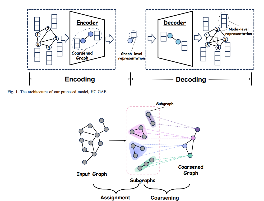
Encoder Link to heading
Encoder consists of a bunch of layers, where each layer can be characterized by two processes:
- Subgraph Assignment
- Coarsening
Subgraph Assignment Link to heading
The idea is that we have an input graph which is compressed into an output graph, by assigning one or more nodes from the input graph to a single node in the output graph. The assignment works in two steps:
- Soft Assignment $$ S_{soft} = \begin{cases} softmax(GNN(X^{(l)}, A^{(l)})) & \text{if } l = 1 \ softmax(X^{(l)}) & \text{if } l > 1 \end{cases} $$
- $S_{soft} \in R^{n_{(l)} \times n_{(l+1)}}$
This just calculates the probability that a node $i$ from the input graphs will belong to node $j$ in the output graph
- Hard Assignment $$ S^{(l)}(i, j) = \begin{cases} 1 & \text{if } S_{soft}(i, j) = \max_{\forall j \in n_{l+1}} [S_{soft}(i, :)] \ 0 & \text{otherwise} \end{cases} $$ Nothing fancy we just take the maximum, this enforces that the input graph is partitioned into a bunch of Subgraphs.
Another view on this problem is that we learn a mapping between two Graph Adjacency matrices:
$$A^{(l+1)} = S^{(l)^T} A^{(l)}S^{(l)}$$
Coarsening Link to heading
Once we have the learned subgraph partitioning, we learn the node representations for coarsened graph:
$$Z_j^{(l)} = A_j^{(l)}X_j^{(l)}W_j^{(l)} $$
This is just Graph Convolution Network (GCN), where we aggregate information from a neighborhood, and since we operate on Subgraphs we do not need to worry about over-smoothing. Given the learned representations we derive the node features:
$$X^{(l+1)} = Reorder[\underset{j=1}{\overset{n_{l+1}}{\parallel}} s_j^{(l)^\top}] Z^{(l)}$$
- $s_j^{(l)} = softmax(A_j^{(l)} X_j^{(l)} D_j^{(l)})$ these are just mixing weights
- we need to REORDER so we use the correct weight with the correct embedding
Final Graph Representation Link to heading
For the final graph representation we usually pool the remaining node representations with some sort of pooling like Mean, Max, Min pooling or other.
Decoder Link to heading
The decoder reverses the graph compression in multiple layers. The key distinction is that we use only soft assignment (with hard assignment we would end up with a bunch of subgraphs) and it is done by learning the re-assignment matrix:
$$ \bar{S}^{l’} \in R^{n_{(l’)} \times n_{(l’ +1)}}$$
- in this case $n_{(l’)} < n_{(l’+1)}$ $$ \bar{S}^{(l’)} = softmax(GNN_{l’, re}(X’^{(l’)}, A’^{(l’)})) $$
And we reconstruct the latent representation of individual nodes:
$$ \bar{Z}^{(l’)} = GNN_{l’, emb}(X’^{(l’)}, A’^{(l’)}) $$
- $GNN_{re}, GNN_{emb}$ are two GNN decoders that do not share parameters
Now we can compute $A^{(l’)}$ the same fashion as in the encoder, but here we increase the dimensions with each layer.
$$ A’^{(l’+1)} = \bar{S}^{(l’)^\top} A’^{(l’)} \bar{S}^{(l’)} $$
And the reconstructed node features: $$ X’^{(l’+1)} = \bar{S}^{(l’)^\top} \bar{Z}^{(l’)} $$
Loss Link to heading
The loss is a bit tricky, we have a local loss, this covers the information in the subgraphs (needs to capture each layer, where the coarsening happens) and a global loss that captures the information in the whole graph.
$$ L_{local} = \sum_{l=1}^{L} \sum_{j=1}^{n_{(l+1)}} KL[q(Z_j^{(l)} | X_j^{(l)}, A_j^{(l)}) || p(Z^{(l)})]$$ $$ L_{global} = -\sum_{l=1}^{L} E_{q(X^{(L)}, A^{(L)})|X^{(l)}, A^{(l)}} [\log p(X’^{(L-l+2)}, A’^{(L-l+2)} | X^{(L)}, A^{(L)})]$$
$$ L_{HC-GAE} = L_{local} + L_{global}$$
- $Z^{(l)}$ a Gaussian prior, introduced
Final Remarks Link to heading
The overall approach of continually compressing the graph, each time splitting a graph into subgraphs and aggregating the information in them is a great way to avoid oversmoothing. What I find personally compelling is the application to domains where there are naturally occurring subgraphs. At code:Breakers I do a lot of AI stuff around source code and cybersecurity. If you think about it, source code is inherently a huge graph, which nicely aggregates: individual statements into control flow, control flow into functions, functions into classes, those into modules. With HC-GAE I can force this natural aggregation into the training objective, and not just that, introduce some extra aggregation along the way to make the final representation as effective as possible.