Conditional independence¶

The most important part of graphical models is the conditional independence assumption.

\[X_A \perp_G X_B | X_C\]

Hence A is independent of B given C in the graph G and is defined as:

Let $I(G)$ be a set of all such CI statements encoded by the graph. We say that $G$ is an I-map (Independence map) for $p$, or that $p$ is Markov wrt $G$, iff $I(G) \subseteq I(p)$ where $I(p)$ is the set of all CI statements that hold for distribution $p$, in other words, the graph is an I-map if it does not make any assertions of CI that are not true of the distribution. This allows a graph to model CI.

In case that a graph is fully connected, it is an I-map of all distributions since it does not make any CI assumptions. Hence we can say that $G$ is a minimal I-map of $p$ if $G$ is an I-map of $p$, and if there is no $G' \subseteq G$ which is an I-map of p.

D-Separation ¶

Allows to reason about CI in graphs. From this we can derive other rules:

Clarify some notation

$\{1,2,3\} \backslash \{1,3\} = \{2\}$$

Directed local Markov property¶

\[t \perp nd(t) \space \backslash \space pa(t) | pa(t) \]

nd(t) are the non descendants of a node ($nd(t) = V \space \backslash \space \{ t \cup desc(t) \}$)

This equation is also known as the directed local Markov property.

Example:

$nd(3) = \{2,4 \}$ and $pa(3) = 1$ hence $3 \perp 2,4 | 1$

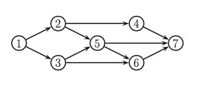
Ordered markov property¶

\[t \perp pred(t) \space \backslash \space pa(t) | pa(t)\]

$pred(3) = \{1,2 \}$ and $pa(3) = 1$ then $3 \perp 2 | 1$

Markov blanket and full conditionals¶

Markov blanket $mb(t)$ of a node t is the set of of nodes that renders the node t conditionally indpendent of the other nodes in the graph.

Markov blanked of a node in a DGM is equal to the parents, children and co-parents (nodes who are also parents of its children)

\[mb(t) \triangleq ch(t) \cup ca(t) \cup copa(t)\]

$mb(5) = \{ 6,7\} \cup \{ 2,3\} \cup \{4\}$

To see why the co-parents are in the Markov blanked we can derive

\[ p(x_t| x_{-t}) = p(x_t, x_{-t}) / p(x_{-t}) \]

All the terms that od not involve $x_t$ will cancel out between numerator and denominator, so we are left with a product of CPDs which contain $x_t$ in their scope:

\[p(x|x_{-t}) \propto p(x_t| x_{pa(t)}) \prod_{x\in ch(t)} p(x_s| x_{pa(s)})\]

Example:

$p(x_5 | x_{-5}) \propto p(x_5| x_2, x_3)p(x_6|x_3,x_5)p(x_7|x_4, x_5,x_6)$

This result is called t’s full conditional distribution

study-notes

Conditional independence¶

D-Separation¶

Directed local Markov property¶

Ordered markov property¶

Markov blanket and full conditionals¶

D-Separation ¶