Directed graphical models
Use directed graphs (DAG) to represent probability distributions.
Also known as
Bayesian network,
Belief networks, they representation is subjective.
Casual network, directed arrows model casual relationship
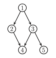
The key property of DAGs is that nodes can be ordered such that parents come before children. Given this ordering we define the ordered markov property, which assume that the children depend only on their parents, not on all the predecessors.
preds(s) are the predecessors of the node s
pa(s) are the parents of node s
Now we can simplify the join distribution of the following graph
Formal definition
Bayesian Network is a directed graph \(G = (V,E)\) together with:
random variable \(x_i\) for each node \(i \in V\)
conditional probability distribution (CPD) \(p(x_i| x_{pa(t)})\) per node, specifying the probability of \(x_i\) conditioned on its parent’s values. (this is often defined as probability tables.)
It defines the following joint probability distribution. $\(p(x_{1:V}| G) = \prod_{t=1}^V p(x_i| x_{pa(t)})\)$
This probability distribution \(p\) defines an I-map (independence map).
If each node has \(O(F)\) parents and K states the number of parameters in the model is \(O(VK^F)\), which is much less than the \(O(K^V)\) needed by a model which makes no CI assumptions.
Examples
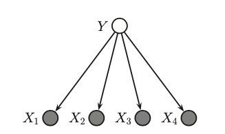
Naive Bayes
In naive bayes we assume that features are conditionally independent given the class label.
Learning
Structure learning Here we try to learn the structure of the directed acyclic graph.