Ordinary Least Squares (MLE)
This is the maximum likelihood estimation for an linear regression model where we maximize the log likelihood:
We assume that the observations are I.I.D, and we prefer minimizing to maximing so we define the negative log likelihood (NNL) which is a convex function:
Now if we assume that the likelihood is Gaussian we get:
\(RSS(w)\) is the sum of squares
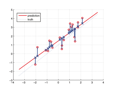
OLS tries to minimize the sum of squares:

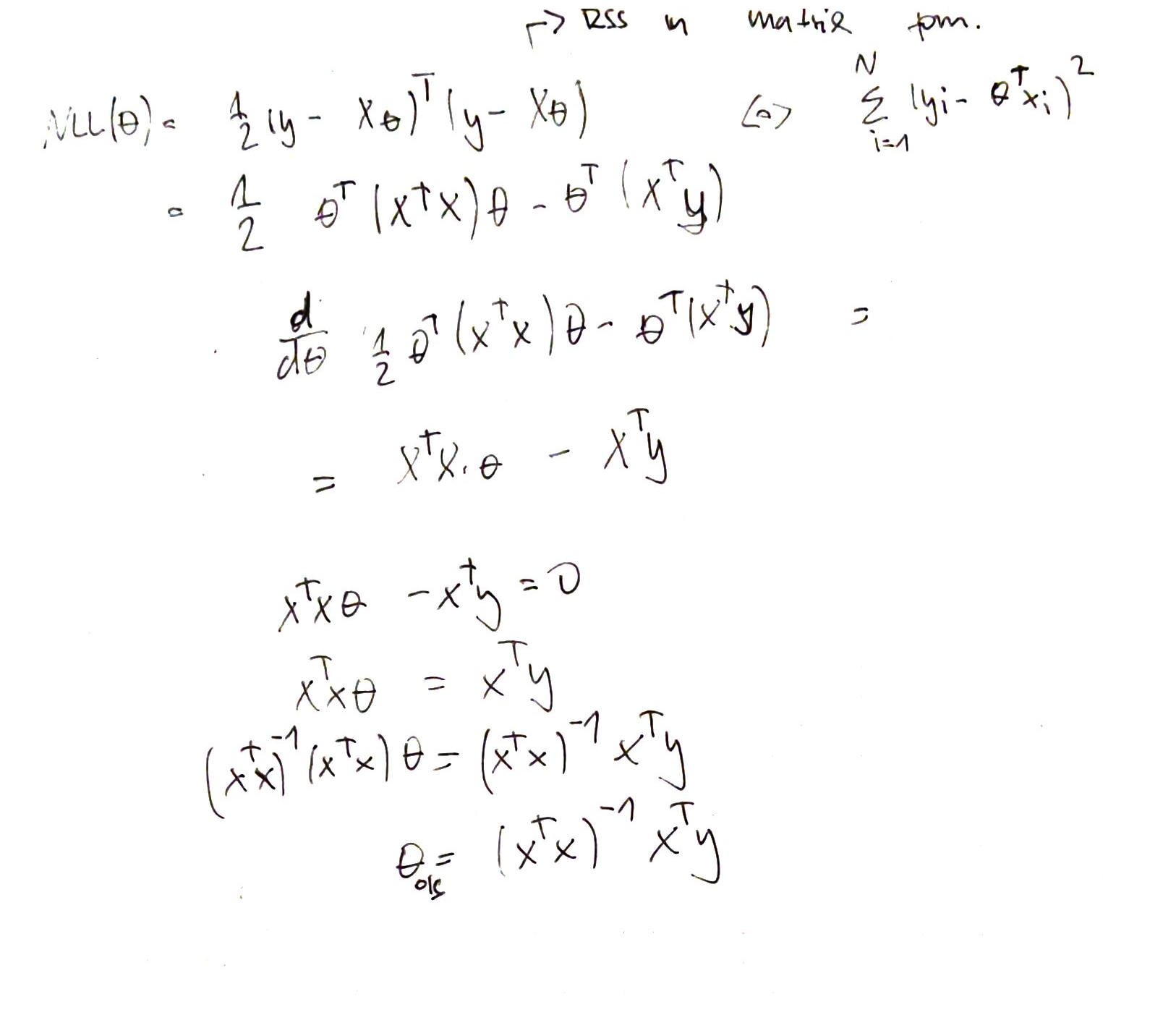
Derivation of MLE (OLS)
Here we derive the ordinary least squares equation:

Geometric interpretation of OLS (MLE)
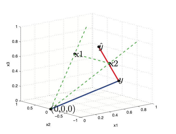
Now if we assume \(N > D\), that meas we have more observations that features. That means that the columns of X define a subspace of dimensionality D which is embeded in N dimensions. This meas that the vector of observed target values \(y\), wil be outside the subspaces spaned by X. Hence our goal is to find a vector \(\hat{y}\) such that is as close to \(y\) than possible.
This can be done, by projecting \(y\) onto the subspace spanned by \(X\). In other words we want to find a linear combination of column vectors of X. \(\hat{y} = w_1 x_1 + \cdots + w_D x_D = Xw\). We define the error vector \(\epsilon = y - \hat{y}\), if this vector will be orthogonal to every column vector of X, than we find the projection \(\hat{y}\) that is closest to the true value \(y\).
If we expand the equation we get:
Now our projected value of \(\hat{y}\) is given as:
This corresponds to an orthogonal projection of y onto the column space of X. Where \(P \triangleq X(X^TX)^{-1}X^T\) is the projection matrix.

