Laplace (Gaussian) approxiation
This is a widely used technique for Gaussian approximation to a posterior distribution. Which is reasonable since the posterior ofthen becomes Gaussian-like as the sample size increases.
We are interested to find the posterior
\(\theta \in R^D\)
\(E(\theta) = - \log p(\theta,D)\) is called the energy function and it is equal to the negative log of the unormalized log posterior
\(Z = p(D)\) is the normalization constant.
If we Tailor expand expand the energy function at the mode \(\theta^*\) we get:
\(g \triangleq \nabla E(\theta)|_{\theta^*}\) is the gradient of the energy function at the mode
\(H \triangleq \frac{\partial^2 E(\theta)}{\partial \theta \partial \theta^T}|_{\theta^*}\) is the Hessian of the energy function evaluated at the mode
Since \(\theta^*\) is the mode, thus the gradient is zero we can simplify this into:
Which is just a Gaussian approximation to the posterior, where the mean of the Gaussian is the mode, and the curvature is given by the inverse of the Hessian at the mode.
This approximation is reasonable since the posterior becomes Gaussian-like if the sample size increases.
Another View
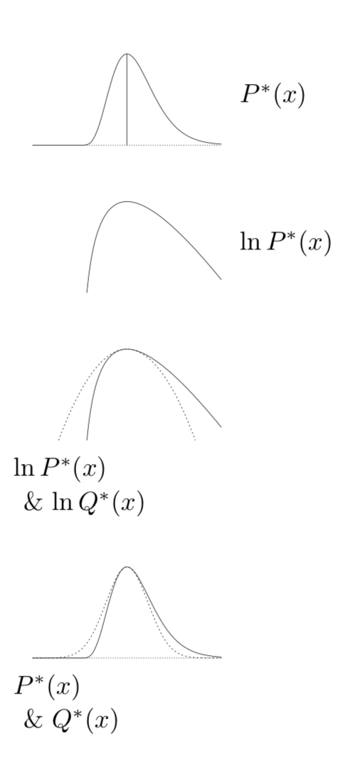
We assume that an unnormalized probability density \(P^*(x)\) whose normalizing constant is:
and has a peak at point \(x_0\). We then Taylor-expand the logarithm of \(P^*(x)\) arround this peak:
where \(c = \frac{\partial ^2}{\partial x^2} \ln P^{*}(x)|_{x = x_0}\)
Then we approximate \(P^*(x)\) by an unnormalized Gaussian
\(Q(x) \equiv P^*(x_0) \exp [- \frac{c}{2}(x - x_0)^2]\)
Next we approximate the normalization constnat \(Z_P\) by the normalizing constant of the Gaussian.
Now we can use Q to make prediction. This is widely-used in physics and it is know as the saddle-point approximation.
The Laplace approximation is basis-dependent: if \(x\) is transformed to a nonlinear function \(u(x)\) and the density is transformed to \(P (u) = P (x) |dx/du|\)
This procedure can be generalized into higher dimension.