Variable elimination algorithm
It is algorithm for exact marginal inference in graphical models.
The main motivation behind variable elimination is to reduce the runtime of inference by leverage factorization of our probability distribution.
Factors
We express an given graphical model as a product of factors.
These factors are:
In Bayesian Networks factors correspond to conditional probability distributions
In Markov Random Fields they encode an unnormalized distribution, to get the marginals we first compute the partition functions using Variable elimination, than we compute unnormalized marginals and than we divide by the partition function.
Factor operations
We repeatedly perform two factor operations
Product
Marginalization
Product operation
We define the product of two factors as a new factor:
The scope of \(\phi_3\) is defined as the union of variables in the scopes of \(\phi_1, \phi_2\)
\(x_c^i\) denotes an assignment ot the variables in scope of \(\phi_i\) defined by the restriction of \(x_c\) to that scope
Example:
\[\phi_3(a,b,c) = \phi_1(a,b)\times \phi_2(b,c)\]
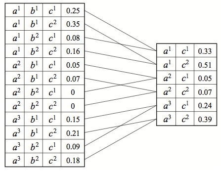
Marginalization operation
Locally eliminates a set of variables form a factor, for example if we have a factor \(\phi(X,Y)\), marginalizing Y produces a new factor:
This makes \(\tau\) a marginalized factor, this marginalized factor in general is not a probability distribution.
Example we have a factor \(\phi(A,B,C\)) and we marginalize over B
Ordering
In variable elimination we need to determine the order in which the variables will be eliminated. (If we perform this elimination on a DAG, we can use the ordering implied by it).
The ordering can have an dramatic impact on the runtime
Finding the best ordering is NP-hard
Algorithm
We loop over variables as ordered by an ordering O, and eliminate them in that ordering. This corresponds to choosing a sum and “pushing it in” as far as possible inside the product of the factors.
For each variable \(X_i\) (ordered according to O)
Multiply all factor \(\phi_i\) containing \(X_i\)
Marginalize out \(X_i\) to obtain a new factor \(\tau\)
Replace the factors \(\phi_i\) with \(\tau\)
Run time
M is the maximum size of any factor \(\tau\) formed during the process
n is the number of variables
Choosing Ordering
Choosing an optimal ordering is NP-hard. Thus we use heuristics:
Min-neighbors: Choose a variable with the fewest dependent variables.
Min-weight: Choose variables to minimize the product of the cardinalities of its dependent variables
Min-fill: Choose vertices to minimize the size of the factor that will be added to the graph.
Cons
An important shortcoming of VE is that we can compute the marginals \(p(Y|E=e)\) for undirected and directed networks, but if we want to ask different queries \(p(Y_2|E=e_2)\) we have to start form scratch.
Fortunately we can tune this by caching intermediate factors \(\tau\) and use them to answer other marginal queries.
There are two common algorithms:
Belief propagation which can be applied to tree-structured graphs
Junction tree algorithm which can be applied to general networks.