PCA for categorical data
We can use this to visualize high dimensional categorical data.
\(W_r \in R^{L \times M}\) is a loading matrix for response \(j\)
\(w_{or} \in R^M\) is offset term for response \(r\)
\(\theta = (W_r, w_{or})_{r=1}^R\)
\(\mu_0 = 0\) s the prior mean (we can capture non zero mean by changing \(w_{0j}\))
\(V_0 = I\) is the prior variance (we can capture non-identity covariance by changing \(W_r\))
Supervised PCA (Bayesian factor regression)
This is a model like PCA but it also takes the target variable \(y_i\) into account when learning the low dimensional embedding.
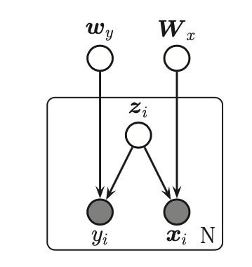
Since the model is jointly Gaussian we have:
\(w = \Psi^{-1}W_xCw_y\)
\(\Psi = \sigma^2_x I_D\)
\(C^{-1} = I + W^T_x \Psi^{-1}W_x\)
Partial least squares
Is a more “discriminative” for of supervised PCA. The key idea is to allow some of the variance in the input features to be explained by its own subspace \(z_i^x\) and let the rest of the subspace \(z_i^s\) be shared between input and output.
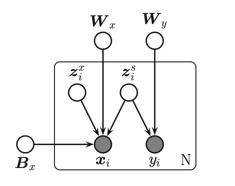
The model:
The corresponding induced distribution on the visible variables has the form:
\(v_i = (x_i ; y_i)\)
\(\mu = (\mu_y ; \mu_x)\)
And:
Canonical correlation analysis
Canonical correlation analysis or CCA is like a symmetric unsupervised version of Partial least squares. It allows each view to have its own “private” subspace, but there is also a shared subspace. If we have two observed variables \(x_i\) and \(y_i\) then we have three latent variables, \(z_i^s \in R^{L_0}\) wich is shared, \(z_i^x \in R^{L_0}\)and \(z_i^y \in R^{L_0}\) which are private. We can visualize the model as:
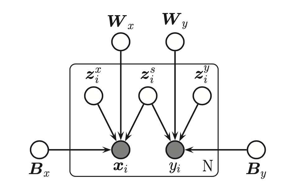
The observed joint distribution has the form:
where