.md .pdf

Contents

Linear discriminant analysis

It is Gaussian model for classification that is similar to Quadratic discriminant analysis where we assume Gaussian distribution for each class, but instead of having specific covariacne matrix for each class $\Sigma_c$ we defined an shared covariance matrix $\Sigma$.

$$p(y=c|x, \theta) \propto \pi_c \exp {[\mu_c^T \Sigma^{-1}x - \frac{1}{2} x^T \Sigma^{-1}x - \frac{1}{2} \mu_c^T \Sigma^{-1}\mu_c] }$$

$$p(y=c|x, \theta) \propto \exp {[\mu_c^T \Sigma^{-1}x - \frac{1}{2} \mu_c^T \Sigma^{-1}\mu_c + \log \pi_c]}\exp{ [- \frac{1}{2} x^T \Sigma^{-1}x ]}$$

The quadratic form:

$$x^T \Sigma^{-1}x$$

is class independent, and it will cancel out the denominator if we define:

$$\gamma_c = -\frac{1}{2} \mu_c^T \Sigma^{-1}\mu_c + \log \pi_c$$

$$\beta_c = \Sigma^{-1}\mu_c$$

Hence we get:

$$p(y = c| x, \Sigma) = \frac{e^{\beta^T_c x + \gamma_c}}{\sum_{c} e^{\beta^T_{c'} + \gamma_{c'}}} = \mathcal{S}(\eta)_c$$

Where:

• $\eta = [B^T_1x + \gamma_1, \cdots, B^T_C x + \gamma_c]$

• $\mathcal{S}$ is the softmax function

For detailed derivation from QDA to LDA

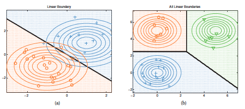
In the context of LDA, if we would take the log of the softmax function we would get a linear function, thus this makes the decision boundary linear.

MLE

If we maximize the log likelihood we get:

$$\hat{\mu}_c = \frac{1}{N_c} \sum_{i: y_i = c} x_i$$

$$\hat{\Sigma}_c = \frac{1}{N_c} \sum_{i: y_i = c} (x_i - \hat{\mu_c})(x_i - \hat{\mu_c})^T$$

$$\hat{\pi_c} = \frac{N_c}{N}$$

Regularization

Mle tends to be ill conditioned (covariance matrix is singular) in high dimensional settings, thus we have to introduce some mechanism to avoid overfitting.

Regularization

We perform MAP estimation on $\Sigma$ using a inverse Wishart Prior of the from $IW(diag (\hat{\Sigma}_{MLE}), v_0)$ hence we have:

$$\hat{\Sigma} = \lambda \text{diag}(\hat{\Sigma}_{MLE}) + (1 - \lambda) \hat{\Sigma}_{MLE}$$

Where:

• $\lambda$ control the amounth of regularizaton.

$$\begin{split}\hat{\Sigma}_{MLE} = V (\frac{1}{N} Z^TZ - \mu \mu^T)V^T \\ X = UDV^T \\ Z = UD\end{split}$$

• $X$ is the design matrix

It is impossible to compute $\hat{\Sigma}_{MLE}$ if $D > N$, (Wide short matrix). But we can use SVD of X.

$X = UDV^T$

Diagonal LDA

If we use regularized LDA but we set $\lambda = 1$ then we get a special variant called Diagonal LDA

Variable elimination motivation Structured predictions