Factor analysis (FA)
One problem with mixture models is that they use only a single latent variable to generate the obervations. One observation can come from one of K prototypes. Since the prototypes are mutually exclusive the model is limited in its representational power.
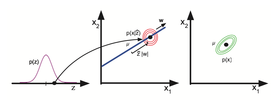
Alternatively we can use an vector valued latent variable \(z_i \in R^L\) and use an Gaussian prior:
If the observations \(x_i\) is are also continuous \(x_i \in R^D\) we may use a Guassian for the likelihood. And as in linear regression we assume that the mean is a linear function of the hidden inputs:
\(W_{D \times L}\) is a factor loading matrix
\(\Psi_{D \times D}\) covariance matrix, and we force it to be diagonal hence it will force \(z_i\) to explain the correlation instead of covariance.
The overal model is called Factor analysis
This model can be viewed as a version of linear factor model
FA as a low rank parametrization of MVN
Factor analysis can be thought as a way of specifying a joint density model on x using a small number of parameters.
\(\mu_0 = 0\) can be set without loss of generality since we can absorb \(W\mu_0\) into \(\mu\)
\(\Sigma_0= I\) can be set without loss of generality, since we can emulate a correlated prior by defining a new weight matrix \(\tilde{W} =W \Sigma_0^{-1/2}\)
The covariance:
Thus FA approximates the covariance matrix of visible vector using a low-rank decomposition:
This parametrization is more efficient uses only \(O(LD)\) parameters instead of the full Gaussian covariance \(O(D^2)\).
Inference of latent factors
We ofthen hope that the latent factors will reveal something interesting about the data. To do that we need to compute the posterior over the latent factors:
\(\Sigma_i\) is actually independent of \(i\) so we drop the subscript, computing reqires \(O(L^3 + L^2D)\) time
\(m_i\) are called the latent scores or latent factors computing requires \(O(L^2 + LD)\) time
Unidentifiability
Similar to mixture mudels FA are also unidentifable.