EM Theory
EM monotonically increases the observed data log likelihood until it reaches a local maximum (or saddle point, although such points are usually unstable).
Expected complete data log likelihood is a lower bound
Consider an arbitrary distribution \(q(z_i)\) over the hidden variables. The observed data log likelihood can be written as follows:
Since \(log(u)\) is a concave function we have the following lower bound:
We denote this lower bound as:
\(H(q_i)\) is the entropy of \(q_i\)
This argument holds for any positive distribution q, and we shoud pick q that yields the tightest lower bound. The lower bound is a sum over i of the following form:
\(p(x_i|\theta)\) is independent of \(q_i\), hence we can maximize the lower bound by setting \(q_i(z_i) = p(z_i| x_i, \theta)\). But \(\theta\) is unknown, so instead we use \(q_i^t(z_i) = p(z_i|x_i, \theta^t))\) where \(\theta^t\) is our estimate parameters at iteration t. This is the output of E step.
Pluggin this in to the lower bound we get:
The first term is the expected complete data log likelihood. The second term is a constant wtr \(\theta\). So the M step becomes :
Since we use \(q_i^t(z_i) = p(z_i| x_i , \theta^t)\) the KL divergence becomes zero so \(L(\theta^t, q_i) = \log p(x_i, z_i|\theta^t)\) and hence
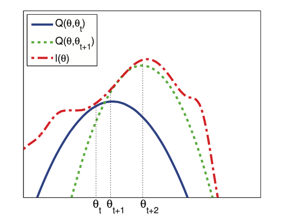
The lower bound is tight after the E step. Since the lower bound “touches” the function, maximizing the lower bound will also “push up” on the function itself. That is, the M step is guaranteed to modify the parameters so as to increase the likelihood of the observed data (unless it is already at a local maximum).

The red dashed curve is the observed log-likelihood. The solid blue curve is the lower bound evaluated at \(\theta^t\), this touches the objective function at \(\theta_t\). We set \(\theta^{t+1}\) to the maximum of the lower bound (blue curve) and fit a new bound at that point (dotted green curve). The maximum of this new bound becomes \(\theta^{t+2}\).
EM monotonically increases the observed data log likelihood
We have:
The first inequality hodls since \(Q(\theta, .)\) is lower bound on \(l(\theta)\). The second is done by definitiion \(Q(\theta^{t+1}, \theta^t) = \max_{\theta} Q(\theta^t, \theta^t)\) .
From this result, if we do not observe monotonic increase of the observed data log likelihood there must be an error. (Code or Math)
