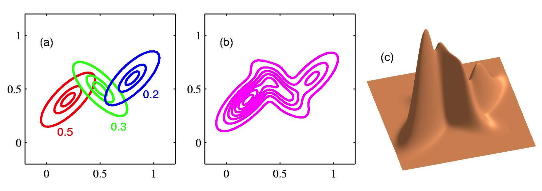
Mixture of Gaussians
The most widely used mixture model is the mixture of Gaussians also known as Gaussian mixture model (GMM). In this model each base distribution is a mixture of multivariate Gaussians with mean \(\mu_k\) and covariance matrix \(\Sigma_k\).
\(\pi_k = p(z=k)\)
\(\sum_k \pi_k = 1\) are the mixture weights
Here we assume that our observed data is comprised of K cluster with proportions specified by \(\pi_1, \cdots, \pi_k\), where each cluster is a Gaussian.

The Gaussian mixture can be viewed as a universal approximator, we can approximate any smooth density with zero error if we have enough components.
EM
One way to fit Gaussian mixture model is to use EM
We assume a known number of K mixture components:
\(r_{ik} = p(z_i = k| x_i, \theta^{(t-1)})\) is the responsibility that cluster k takes from data point i.
E step
This is the same for all mixture models
M step
We need to optimize Q with respect to \(\pi\), \(\mu\) and \(\Sigma\)
\(r_k = \sum_i r_{ik}\) the number of points asigned to cluster k
For \(\mu_k, \Sigma_k\) we simplify Q and leave only the parts it depends on
This is just the weighted MLE of an NVM
This is intuitive the mean of cluster \(k\) is just the weighted average of all points assigned to cluster k, and the covariance is proportional to the weighted empirical scatter matrix.
Now we set \(\theta^k = (\pi_k, \mu_k, \Sigma_k)\) for \(k = 1 : K\) and go to the next E step.
