Ridge regression (Penalized least squares)
The MLE can easily overfit, since it tries to fit the data as best as possible, thus it results in complex functions. Example of ordinary least squares up to a 14 degree polynomial:
We get the following weights:
6.560, -36.934, -109.255, 543.452, 1022.561, -3046.224, -3768.013, 8524.540, 6607.897, -12640.058, -5530.188, 9479.730, 1774.639, -2821.526
Here we that we have many large positive and negative numbers. They balace each out thus resulting in a wiggly curve, that nearly perfectly interpolates the data. However this is guaranteed to overfit. To reduce overfitting we have to encourage these parameters to be small. A simple way of doing this is to put a Gaussian prior on our parameter estimation:
\(1/\tau^2\) control the strenght of the prior.
If we put this together than we have the corresponding MAP estimation problem:
Or equivalently we can express it as a minimization problem, where our loss function is:
\(\lambda \triangleq \sigma^2 / \tau^2\) is the complexity penalty.
\(||w||_2^2 = \sum_jw^2_j\) is the squared two-norm
Hence our estimate for \(w\) is:
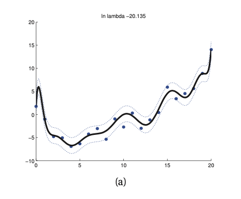
\(\lambda\) constrols the complexity choosen in cross-validation.
we do not need to penalyze \(w_0\) since it just affect the height of the function it do not contribute to complexity.
by penalizing the sum of magnitues of the weights, we ensure the function is simple (w = 0 corresponds to a straight line, which is the simplest possible model).
This naive way is not numerically stable