Markov models
Idea behind a Markov chain is to assume that \(X_t\) (current state) captures all the relevant information for predicting the future. We can express it as the following joint distribution:
This is called a Markov chain or Markov model.
If we assume that the transition function \(p(X_t| X_{t -1})\) is independent of time, then the chain is called homogeneous, stationary, or time-invariant. This is an example of parameter tying, since the same parameter is shared by multiple variables. This assumption allows us to model an arbitrary number of variables using a fixed number of parameters; such models are called stochastic processes.
If we assume that the observations are discrete, we get a discrete-state or finite-state Markov chain. Most of the models are discrete.
Transition matrix
When \(X_T\) is discrete os \(X_t \in \{1, \cdots, K \}\) the class conditional distribution \(p(X_t| X_{t-1})\) can be written as a \(K \times K\) matrix known as the transition matrix A, where \(A_{ij} = p(X_t = j | X_{t-1} = i)\) is the probability going from state i to state j. If each row of the matrix sums to 1 we have a stochastic matrix.
A stationary, finite-state Markov chain is equivalent to a stochastic automaton. It is common to visualize such automata by drawing a directed graph, where nodes represent states and arrows represent transitions.
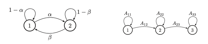
The latter is an example of left to righ transition matrix
\(A_{ij}\) represents the probability of getting from i into j in one step. The n-step transition matrix \(A(n)\):
If is the probability of getting from i to j in exactly n steps. Then Chapman-Kolmogorov equations states that:
Which is the probability of getting from i to j in m + n steps is just the probability of getting from i to k in m steps and then from k to j in n steps summed up over all k. We can express it as matrix multiplication:
We can simulate multiple steps of a Markov chain by “powering up” the transition matrix.
Stationary distribution of a Markov chain
We can interpret a markov chain as a stochastic dynamical system, where we hop from one state to another at each time step. In this case, we are often interested in the log term distribution over states, which is known as the stationary distribution.